Merge a composite first
To merge microscopy channels in ImageJ, open the separate grayscale images, choose Image > Color > Merge Channels and enable Create composite. Keep the source images, check each channel in the result and save a composite TIFF before making an RGB presentation copy. A composite keeps channel planes separately accessible; an RGB copy stores the rendered red, green and blue components. Splitting that RGB copy cannot recover the original 16-bit acquisition values.
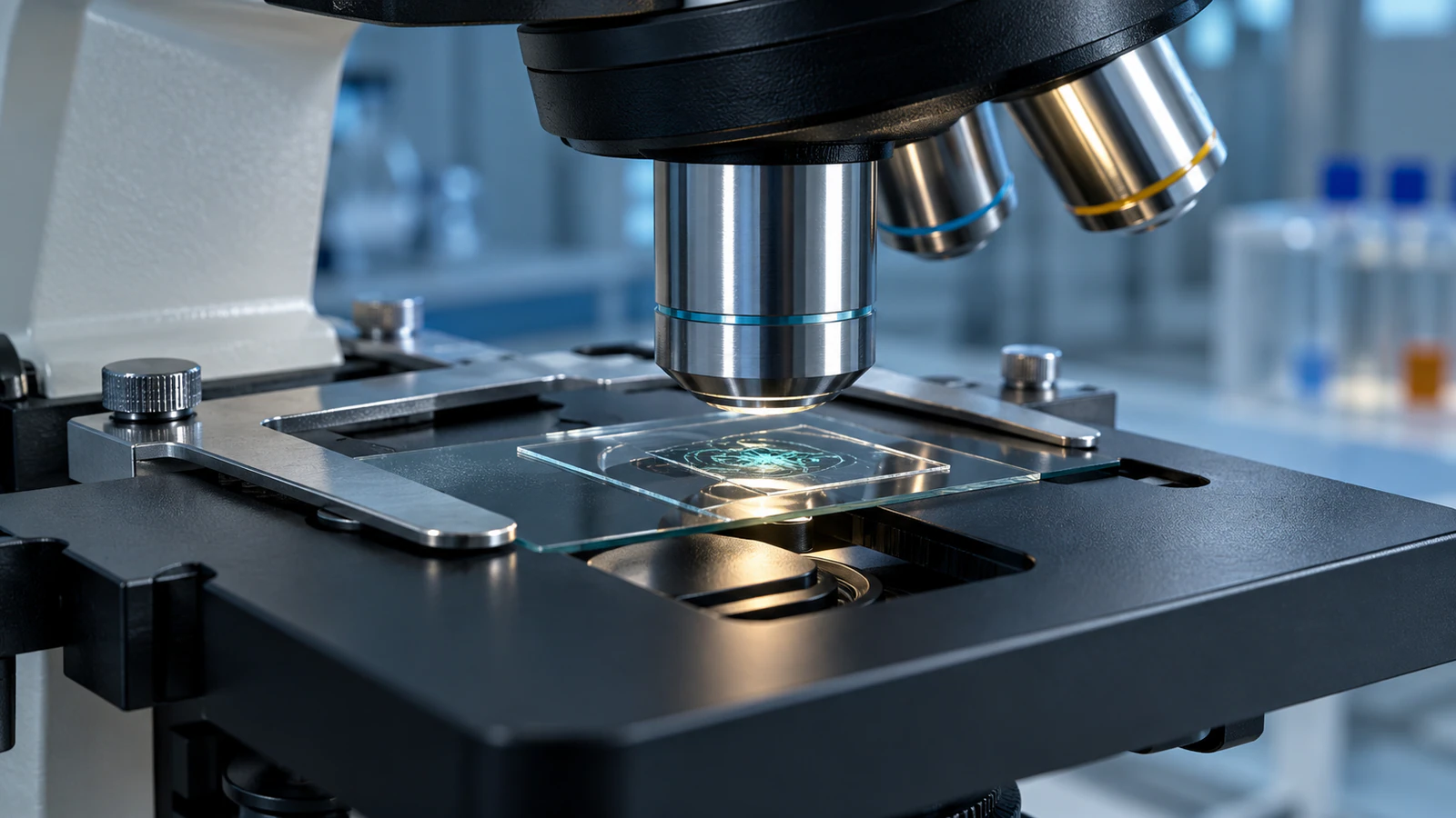
This guide follows one small, reproducible example through that boundary. Two synthetic channels are merged, saved, reopened and converted to RGB. The audit was executed in ImageJ 1.54g using its macro language; the menu descriptions were checked against the official documentation. These are software tests, not biological measurements. The four illustrations are conceptual CGI and are not screenshots or microscopy evidence.
Check the files before assigning colors
Work on copies and retain the acquisition files, including their metadata. The Office of Research Integrity guidance on originals explains why a processed figure cannot replace that record. An ImageJ TIFF is a useful working file, but it is not a promise that every vendor-specific metadata field survives conversion.
For this procedure, prepare two single-channel grayscale images with matching width, height, bit depth and corresponding planes. Confirm that they show the same field, z position and time point. Equal dimensions do not establish registration: two unrelated 512 by 512 images can still merge into a convincing picture.
If the input already contains multiple channels, inspect its channel, slice and frame dimensions before splitting anything. A channel axis records different signals; a z axis records depth; a time axis records successive observations. Mistaking one for another can produce a plausible-looking but incorrect combination. Keep the original acquisition channel names in a separate record.
Choose colors without changing identity
A lookup table, or LUT, maps grayscale values to display colors. In a fluorescence composite, that color is a viewing choice rather than the identity of the measurement. Keep a written mapping such as “channel A: nuclear marker, magenta” and “channel B: mitochondrial marker, green.” Those marker assignments are an illustrative planning example here, not the contents of our synthetic test.
Use the same mapping in individual-channel views, the merge and the caption. Include grayscale single-channel panels when readers need to inspect the underlying patterns. A viewer should not have to infer a marker from a familiar color convention.
Do not interpret a pale overlap region as proof that proteins bind. The ImageJ colocalization guide explains why visual color overlap is an inadequate analysis. Registration, spectral bleed-through, resolution and the experimental question still matter. Our colocalization and interaction guide develops that distinction for explanatory visuals.
Set up the merge deliberately
Assign the intended LUT to each source image and choose its display range before merging. For the synthetic test, both ranges are 0 to 3000, with magenta for A and green for B. Equal display limits are convenient for this test; they are not a general normalization method for different fluorophores or acquisition settings.
Open Image > Color > Merge Channels. Put image A in C1 and image B in C2, leaving unused slots empty. Enable Create composite and Keep source images. Leave Ignore source LUTs off when you want the source LUTs and display ranges retained. The Merge Channels documentation describes these controls.
Inspect the result with Image > Color > Channels Tool. Toggle the two channels individually, then together. Confirm their order and colors before continuing. If the display looks wrong, compare the source windows and display ranges first; a change in appearance does not automatically mean the pixel data changed.
Reproduce the two-channel test
Use a fresh ImageJ session with no valuable unsaved images. Open Plugins > New > Macro, enter the following lines in order and run the macro. The example creates two four-pixel, 16-bit images. The numbers are deliberately small enough to inspect one by one and have no physical units.
The macro function reference documents newImage, setPixel and setMinAndMax. The Plugins menu guide describes the macro editor and recorder. For a differently configured installation, record your own Merge Channels operation and compare its options before applying it to a dataset.
- newImage("A", "16-bit black", 4, 1, 1);
- for (x=0; x<4; x++) setPixel(x, 0, 1000*x);
- run("Magenta");
- setMinAndMax(0, 3000);
- newImage("B", "16-bit black", 4, 1, 1);
- for (x=0; x<4; x++) setPixel(x, 0, 3000-1000*x);
- run("Green");
- setMinAndMax(0, 3000);
- run("Merge Channels...", "c1=A c2=B create keep");
Compare values before trusting the display
Our audit produced a 4 by 1 image with two channels, one z slice and one time point. Each channel remained 16-bit. The magenta LUT ended at RGB 255, 0, 255; the green LUT ended at 0, 255, 0. Both display ranges remained 0 to 3000.
After saving the composite as TIFF and reopening it, every value below was unchanged. The two channels and their LUT endpoints were also retained. This verifies this particular ImageJ round trip, not every microscope format, plugin or downstream application. Repeat the check on representative files from your own workflow.
A practical audit should sample a dim pixel, a bright pixel and a region with structure, then compare the same coordinates before and after saving. Record channel selection as well as x and y. A value read from the wrong active channel can look like data corruption even when the file is intact.
| Pixel x | A before and after TIFF | B before and after TIFF |
|---|---|---|
| 0 | 0 | 3000 |
| 1 | 1000 | 2000 |
| 2 | 2000 | 1000 |
| 3 | 3000 | 0 |
Save an editable file and a presentation copy
Save the checked composite with File > Save As > Tiff, close it and reopen it in ImageJ. Confirm channel count, bit depth, LUTs and display limits. Keep the source files as well. The ImageJ file documentation describes its save operations, while the image types guide distinguishes multichannel data from RGB color.
Duplicate the reopened composite for presentation, then use Image > Type > RGB Color on that copy. In our test, this produced a 24-bit RGB image with one image channel. Its four pixels were (0,255,0), (85,171,85), (171,85,171) and (255,0,255). These are rendered color components, not the original 0 to 3000 channel intensities.
Save that copy as PNG for a slide or figure, subject to the destination requirements. Splitting our RGB copy produced 8-bit color components. The operation did not restore the two original 16-bit signals. Keep analysis attached to the retained data, even when a presentation file looks identical on screen.
Troubleshoot the specific failure
Start with the earliest point where the result diverged from the source. Compare one plane and one channel before investigating an entire experiment. Save a note about any correction, especially a registration transform or a change in display range.
The brightness and contrast guide provides a separate numeric display audit. Check spatial calibration with the ImageJ scale-bar workflow before adding a scale bar to a resized presentation copy.
| Symptom | Check | Action |
|---|---|---|
| Colors change during merge | Ignore source LUTs and source LUT assignments | Retain or deliberately reassign LUTs, then verify channel identities. |
| One signal disappears | Channels Tool selection and active-channel display range | Show each channel alone and compare it with its source. |
| Edges are displaced | Field, crop origin, z plane, time and registration | Return to matched data; do not drag one channel until it looks persuasive. |
| Only 8-bit components remain after splitting | Whether the source was already RGB | Reopen the original acquisition or composite TIFF. |
| Result looks different in another application | Its support for multichannel TIFF and LUT metadata | Use the verified RGB copy for presentation and retain the composite for inspection. |
Write a caption someone can audit
A useful caption identifies the measured channels, their display colors, the spatial view and relevant processing. State whether the image is a single optical plane or a projection, and identify any crop, registration or display adjustment needed to interpret it. Do not call a composite a quantitative colocalization result merely because it contains an overlap color.
For a real dataset, complete a record like this: “Marker A is shown in magenta and marker B in green. The merge shows [specified plane or projection] from [sample and condition]. Display ranges were [values and comparison policy]. [Registration or other processing] was applied. Original channel data and the composite TIFF were retained.” Replace every bracket with an actual fact before publication.
For our synthetic example, the appropriate caption is simpler: “Two invented four-pixel channels test file preservation. No biological specimen was imaged.” This also explains why the surrounding cell illustrations cannot serve as evidence for the numerical result.
- Retain acquisition filenames, import settings and software versions.
- Record channel order, LUTs, display ranges and C/Z/T dimensions.
- Keep the reopened TIFF audit beside the final presentation export.
- Check the exported figure at its actual reading size, including captions and scale bars.
Build a separate cellular explanation
When a lab meeting also needs a mechanism explanation, keep that animation separate from the microscopy result. Animiotics currently supports describing a scientific scene, revising it and editing the camera, colors and timing. A conceptual cell scene can explain spatial relationships; this workflow does not reconstruct a cell from your channel images or calculate colocalization.
Try this scene brief: “Show a simplified mammalian cell with one nucleus and several separate mitochondria. Keep their identities consistent. Begin with an oblique view, then rotate toward a projection-like view where some silhouettes overlap. Rotate back to reveal their different depths. Do not depict binding, measured fluorescence or a reconstructed specimen.” This is a proposed teaching brief, not an Animiotics output tested in this article.
Review the animation against the actual teaching claim. The camera transition should explain why a two-dimensional view can conceal depth. It should not imply that all microscopy overlap is a projection artifact. Keep the measured figure visible as its own evidence and label the animation as an illustration.
Frequently asked questions
Why should I enable Create composite?
It keeps the merged signals in separately accessible channel planes. In our ImageJ 1.54g test, two 16-bit sources remained two 16-bit channels after a TIFF save and reopen. Check your own files rather than assuming every export preserves that structure.
Why did my magenta channel become red?
Check whether Ignore source LUTs was enabled or an RGB merge was created directly. Inspect the source LUT and the resulting channel assignment. A changed display color alone does not identify whether the underlying values changed.
Can I recover fluorescence measurements by splitting a PNG?
Splitting an RGB PNG separates its rendered red, green and blue components. It does not recreate the original higher-bit-depth acquisition channels or undo the display mapping. Use the retained source or composite data.
Does a white or yellow overlap region prove interaction?
No. Its appearance depends on display colors and intensities. Assess the imaging controls, registration, resolution and an analysis appropriate to the biological question before making a colocalization claim, and do not equate colocalization with molecular binding.
Was this procedure tested in Fiji?
The numerical merge, TIFF round trip and RGB conversion were executed in standalone ImageJ 1.54g. The menu procedure was source-checked. Fiji distributions include ImageJ functionality, but their import plugins and versions can differ, so repeat the small audit in your installation.
Try a cellular scene in Animiotics
Use the checked channel figure for your result and try Animiotics for the separate nucleus-and-mitochondria explanation. Review the current trial terms on the homepage before starting. Sign-up and the manual editor are free; AI generation and exports require a paid plan. Inspect the scene for scientific meaning before sharing it.